Skip to content
Rupak Dey

Navigate

Work

Links

Theme

Projects

Engineering

Brain Tumor MRI Classification

Role
The Vision Transformer, the evaluation harness, and the GAN augmentation
Period
Feb 2026 – May 2026
Stack
  • Python
  • PyTorch
  • ResNet-50
  • ViT-B/16
  • Scikit-learn
  • Streamlit

Context#

The task is four-way classification of 2D brain MRI slices: glioma, meningioma, pituitary, and no tumor. It ran twice, once as the four-way problem and once collapsed to tumor against no tumor. The data is Masoud Nickparvar's Brain Tumor MRI Dataset on Kaggle, itself a merge of three upstream collections.

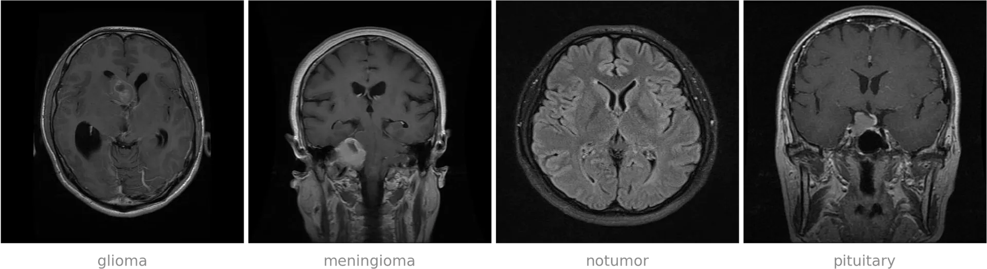
Four brain scans side by side, labelled glioma, meningioma, notumor and pituitary. The glioma is an axial slice with a small bright ring near the centre and dark ventricles. The meningioma is a coronal slice with a rounded bright mass low on the left near the skull base. The notumor slice is symmetric with clear grey and white matter and no lesion. The pituitary is a coronal slice with a small bright mass at the centre of the skull base, eye sockets and sinuses visible.
One image per class, each chosen as the closest to its class mean rather than the most dramatic example. Note that the four are not all the same view: two are axial and two coronal, and the dataset mixes planes freely inside a single class.

Five model families, deliberately spread apart so the comparison would mean something: a Random Forest over HOG and LBP features, a custom CNN with squeeze-and-excitation blocks at 6.6M parameters, a fine-tuned ResNet-50 at 24M, a fine-tuned ViT-B/16 at 86M, and a class-conditional GAN generating extra training data. Eleven runs, about a hundred minutes total on one H100.

The best result was 0.9575 accuracy on the held-out test split. That is the number on the report we submitted, and it does not survive contact with the artifacts behind it. Everything below comes from going back through those artifacts afterwards, which is the only part of this project worth writing down.

Worth being precise about my share before making any claims on it. This was a four-person team, and the final tree landed in three bulk commits from my account, so git blame credits me with 98.7% of the source and is measuring packaging rather than authorship. By commit count Mario Saenz contributed more than I did, and the preprocessing module is a descendant of Mario's file, not mine. What is actually mine is the ViT work, the evaluation harness, the GAN augmentation pipeline, and the inference GUI.

Seven percent of the test set was already in training#

The dataset in the repo is not the stock download. It had been rebalanced by hand to exactly 1400 training and 400 test images per class, against a canonical 7,023, and no script in any of the 35 commits performs that rebalancing. Somebody copied files until the classes came out even.

The tell is that a file-level checksum finds nothing wrong. Hash the JPEG bytes and every image in the repo is unique, which is what you would check first and what makes the problem invisible. Hash the decoded pixel array instead and 114 test images, 7.125% of the split, are byte-identical to an image the model trained on. The containers differ; the pictures do not.

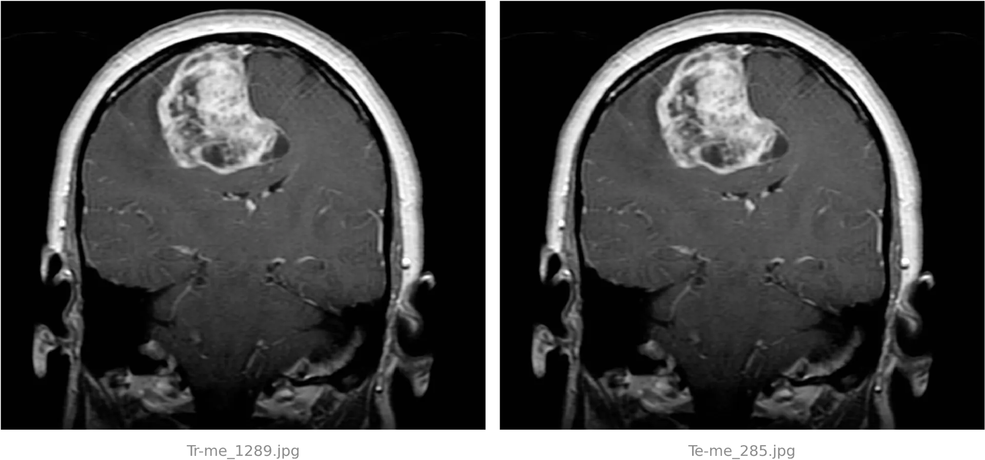
Two identical coronal brain scans side by side. Each shows a head in cross section with a large bright irregular mass in the upper left of the brain, about a third the width of the skull, with a darker cavity at its lower edge. The filename beneath the left panel reads Tr-me_1289.jpg and beneath the right, Te-me_285.jpg.
One of the 114. The same picture, in training on the left and in test on the right, down to the last pixel: both decode to md5 f273fd56f2f765fa32bf7c4161784e47. Their JPEG files do not match, which is the entire reason a file-level sweep reports the split as clean.
file-level md5 over 7,200 JPEGs        0 duplicates
pixel-level md5 over decoded arrays    114 test images already in train
  meningioma 100, notumor 9, glioma 5
cosine >= 0.99 against any train image 455 of 1,600  (28.4%)
  same threshold, different class        2 of 1,600  ( 0.1%)

That last line is the one that makes the rest of it hold up. Brain MRIs all look broadly alike, so a near-duplicate threshold could easily be measuring nothing but generic head shape. Running the same query against training images of a different class returns 2 hits out of 1,600. The threshold discriminates.

Every model scores at or near 1.0000 on the leaked images, which is what memorization looks like from the outside. Recomputing the headline over the 1,145 test images with no near-duplicate:

                 reported   on leaked   clean subset    delta
resnet50_aug      0.9575      1.0000       0.9424      -0.0151
resnet50          0.9487      1.0000       0.9319      -0.0168
vit               0.9487      0.9912       0.9310      -0.0177
custom_cnn        0.9450      0.9737       0.9275      -0.0175
baseline_rf       0.8806      1.0000       0.8358      -0.0448

The clean-subset column is indicative rather than a drop-in replacement, since removing duplicates guts the per-class support unevenly: notumor falls from 400 test images to 58. But the direction and the rough size of the correction are not in doubt.

The same pattern shows up one step earlier, in the splits the models trained against:

train accuracy, final epoch          0.9971
validation accuracy, final epoch     0.9902
test accuracy, as reported           0.9575
test accuracy, near-duplicate free   0.9424

Training and validation are both carved out of the vendor's training directory by a file-level split, so whatever duplication sits in that pool is spread across both sides of it. Test comes from a separate directory. The number falls at every step away from the training pool, in exactly the order you would predict if duplication were doing the work.

The part I find genuinely instructive is where the contamination came from. Perfect class balance is the feature of this dataset that looks most professional in a summary table, and it is exactly what caused the problem. Balance was bought by duplicating images, and the duplicates crossed the split.

The GAN that generated four images#

The augmentation model is a class-conditional DCGAN with spectral normalization on the discriminator, hinge loss, two-timescale updates, and an EMA generator. Trained 80 epochs. Run with --gen-per-class 500, it was supposed to contribute 2,000 synthetic training images, and the run that used it posted the best score in the project.

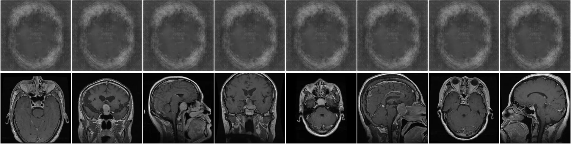
Loading the saved generator and sampling 64 latent vectors per class gives a mean pairwise cosine similarity between samples of 0.9999, in all four classes. The generator ignores the latent code completely. It is a lookup table with four entries.

Two rows of eight greyscale panels. The top row is eight outputs from the trained generator: soft blurred grey ovals on dark backgrounds, faintly suggesting a skull outline, with no internal anatomy and no visible lesion, and all eight are indistinguishable from one another. The bottom row is eight real pituitary training scans, sharply detailed and all different: three axial views through the skull base showing eye sockets and sinuses, three sagittal mid-line views showing the corpus callosum and brain stem in profile, and two coronal views, several with a bright lesion at the pituitary fossa.
Top row: eight draws from the generator, from eight near-orthogonal latent vectors with mean pairwise similarity 0.0158. Their outputs have mean pairwise similarity 0.9999. Bottom row: eight real images of the same class, at 0.6774. Identical greyscale mapping on both rows, no per-image normalization. The class is pituitary, which has the most visually diverse real images of the four.

So --gen-per-class 500 did not add 2,000 samples. It added four distinct images, each duplicated 500 times. In binary mode it added 1,000 copies of a single image labelled no_tumor. The saved sample grid from epoch 80 agrees with the arithmetic: blurred grey ovals, no visible tumor, nothing distinguishing one row from another. The loss trace agrees too, with the discriminator winning decisively by the end.

What makes this worth publishing rather than quietly deleting is that the experiment appeared to work. GAN augmentation improved multiclass accuracy by 0.88 points and binary by 0.31, and those are the numbers in our report, under a section arguing that synthetic samples preserve class-specific information. They do not, and this generator never produced any. The gain is a single-run difference produced by pasting four blurry blobs into the training set several hundred times each, and it is well inside the noise of an experiment nobody ran twice.

There is a second confound underneath the first. The GAN-augmented run is the only one of the four whose best validation loss lands on its final epoch, so it stopped because it ran out of epochs while still improving. The plain ResNet-50 peaked at epoch 10 and was stopped by patience eight epochs later. Whatever separates those two scores, it is not cleanly the synthetic data.

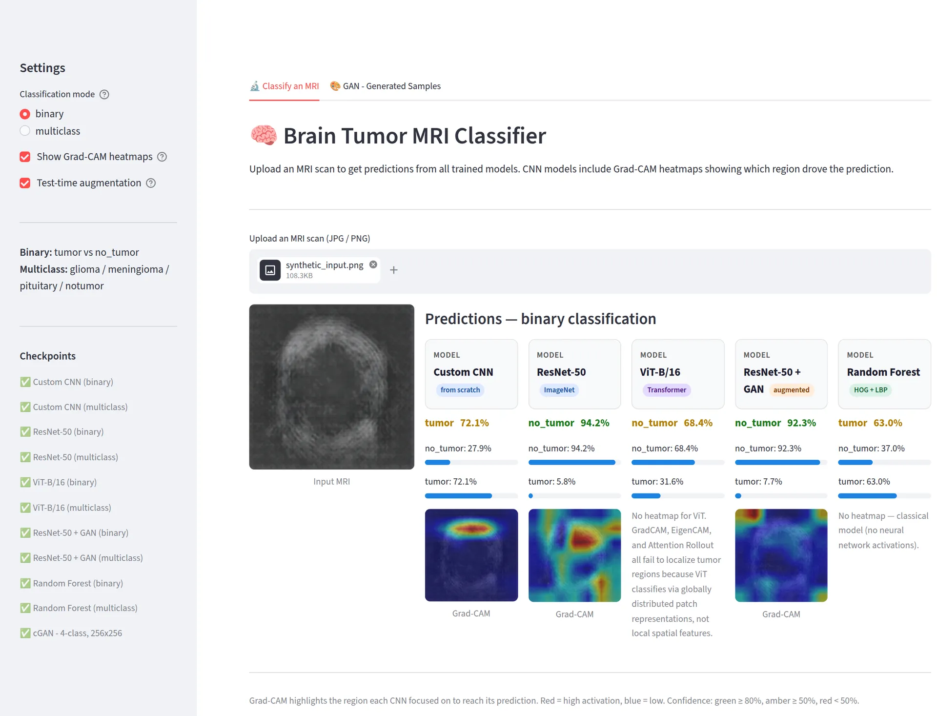
The inference app makes the same point from the other end. Hand it one of the generator's own images and the five classifiers split three to two on whether there is a tumor, at confidences running from 63% to 94%, on a picture that contains no anatomy at all. Confident disagreement is exactly what an out-of-distribution input should produce, so this is not a scandal on its own. It is a preview of the next section.

A two-column inference app. The left sidebar holds a classification mode selector set to binary, checkboxes for Grad-CAM heatmaps and test-time augmentation, the binary and multiclass label sets, and a list of eleven loaded checkpoints. The main panel shows an uploaded input image, a blurred grey oval, beside five model cards: Custom CNN says tumor at 72.1%, ResNet-50 says no_tumor at 94.2%, ViT-B/16 says no_tumor at 68.4%, ResNet-50 plus GAN says no_tumor at 92.3%, and Random Forest says tumor at 63.0%. Three cards carry a blue-to-red Grad-CAM heatmap beneath them.
The input is the collapsed generator's own output, so there is nothing in it to find. The heatmaps are Grad-CAM and are illustrative only: the dataset ships no segmentation masks, so there was never any ground truth to score attention against. The ViT panel, asserting that three attribution methods fail to localize, is the app repeating a claim from our report that no code in the project supports.

A plausible method, a metric that seemed to confirm it, and a saved artifact that disproves both. The artifact was in the repo the whole time.

Glioma, and the limit that was never the model#

Set the leakage aside and one result stays interesting. Here is the best model's confusion matrix on the four-way problem, rows true and columns predicted:

              glioma  mening  notumor  pituit     recall
glioma           335      44       21       0     0.8375
meningioma         0     399        0       1     0.9975
notumor            0       0      400       0     1.0000
pituitary          0       2        0     398     0.9950

Three classes are effectively solved and glioma is not, and capacity does not move it. Per-class recall on the four-way problem, every model, test split:

                 glioma  mening  notumor  pituit
resnet50_aug     0.8375  0.9975   1.0000  0.9950
resnet50         0.8150  0.9925   0.9925  0.9950
vit              0.8125  0.9875   1.0000  0.9950
custom_cnn       0.8075  0.9725   1.0000  1.0000
baseline_rf      0.6675  0.8800   1.0000  0.9750

Every model is worst on glioma and at or near perfect on no-tumor. Across the five families the spread is 0.1700 on glioma and 0.0075 on no-tumor. ViT-B/16 carries thirteen times the custom CNN's parameters and buys 0.005 of glioma recall with them. A Random Forest over hand-crafted HOG features, doing no representation learning whatsoever, fails in the same direction as everything above it.
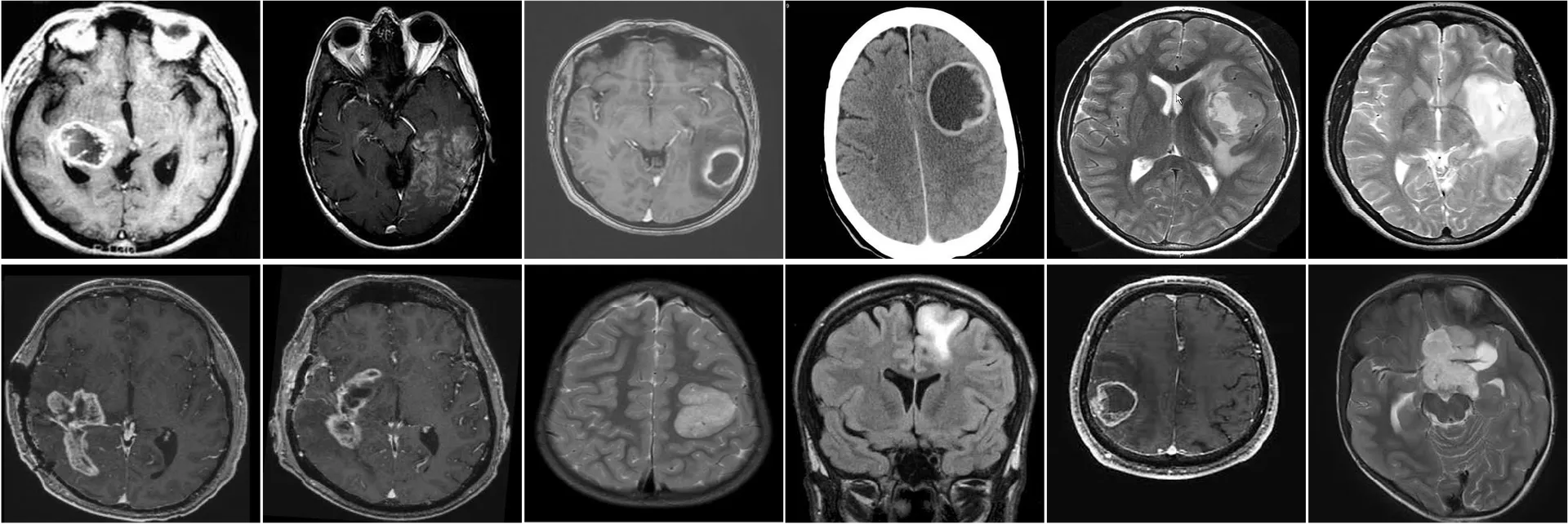
So the limit is not in the architecture, and the images are worth opening.

Twelve brain scans in two rows of six, all gliomas the best model classified as having no tumor. Every panel carries a large obvious lesion. They vary widely in appearance: bright grainy scans, dark scans with bright tissue at the skull base, pale flat-background scans, one with a thick solid white skull ring around a smooth grey brain and a large dark cavity, several bright images with pale masses, and one coronal view with a mass in the upper left frontal region. One panel has faint illegible text burned into the bottom edge and another shows a small mouse cursor near the mid-line.
Twelve of the 21 gliomas the best model called no-tumor. The lesions are not subtle; the images are not consistent. The fourth panel on the top row is the clearest case of the pattern below.

The obvious guess is that these are the subtle tumors, the small or low-contrast ones. The picture refutes that immediately. Nearly every one carries a large, unmistakable lesion, and several are among the most dramatic tumors in the test set. Whatever is failing here, it is not conspicuity.

What the failures share is that they do not look like the training distribution as images, independent of the tumor in them. Set against the 335 gliomas the same model got right, they are roughly twice as bright on average, carry five times the bright-area fraction, and hold 57.8 times the fraction of near-saturated white pixels. Seven of the 21 are more than 2% saturated, where 1 of the 335 correct ones is.

The fourth panel on the top row shows what that means concretely: a thick uniformly bright skull ring around a granular brain, which is what a CT looks like and is not what an MRI looks like. At least three of the 21 have that appearance. Worth being careful about how hard to push it, since the dataset ships no DICOM headers and states no modality anywhere, so this is a reading of pixels rather than an established fact. The rest divide into bright-lesion-on-dark images in a collection whose dominant appearance is the reverse, and a couple of slices in a plane most of the others are not.

The honest summary is that the model does not fail on hard tumors. It fails on unfamiliar image types, and no-tumor is what it emits when an image resembles nothing it was trained on. That is a more interesting failure than subtlety, and the one that would actually matter in use, where scanner and protocol drift is the normal condition rather than the exception. These are also not clustered in any filename range, so they are not one contaminated batch from a single upstream source.

One last thing about those 21. They are only 19 distinct images: two pairs among them are pixel-identical to each other, and both pairs sit inside the test set. Two of the model's worst failures are the same picture counted twice, in a test split that already shares 114 images with training.

What this shows#

The spread across the four deep architectures is 0.0125, from 0.9450 to 0.9575. The leakage correction moves any single one of them by 0.0151. The contamination in the data had a larger effect on the reported number than the entire choice of architecture did, which is a reasonable summary of where the effort in this project should have gone and did not.

Three caveats travel with every number above and cannot be dropped:

Everything is a single run. SEED = 42 is set, cuDNN determinism is not, and each configuration was trained exactly once. Quoting four decimal places implies a precision that no part of this experiment established, and the GAN's 0.88-point "improvement" is unfalsifiable for the same reason.

The binary results need their floor. 0.9831 reads as near-perfect skill until you notice the binary split is 1,200 tumor against 400 no-tumor, so always guessing tumor scores 0.7500. The real gain is 13.31 points, not 98.

The Random Forest baseline is not a fair comparison, twice over. It was selected by looking at test accuracy, and it trained on 5,600 images where the deep models trained on 4,480.

And the thing that should be obvious but is worth writing anyway: this is coursework on 2D slices from a public dataset, never evaluated against radiologist reads and never run on clinical data. It is not a diagnostic tool, and no number on this page should be read as evidence that it could become one.